Homography for tensorflow

Homography for tensorflow

Homography

In the pinhole model, if we care to use homogeneous coordinates, the points in space are projected on the image plane (of the idealized camera sensor) using a simple linear transformation. We would need the 3x4 camera matrix C, which is obtained by putting the camera intrinsic and extrinsic together. The formula for projection will be

To get the non-homogeneous coordinates $u, v$ on the image plane, we rescale everything by $\tilde{w}$

We can use this fact to rewrite the projection as

Here we chose $\lambda$ to have the last parameter of the camera matrix as 1. Notice we will end up again with the same $u, v$ ($\lambda$ cancels out) as you can see

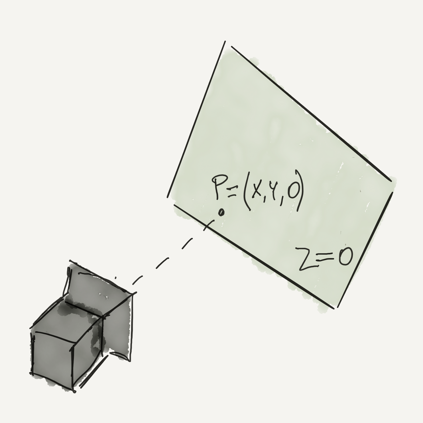
Now consider a plane in the world space, and imagine we aligned the reference system in a way Z=0 for all points on this plane.

For all the points lying on the plane, we can use a simplified version of the projection. The third column of the camera matrix will be irrelevant (multiplied by Z=0 in fact). So we can simplify and write

The projection for a given plane in the world space to the image plane of the camera is called homography and can be expressed by a 3x3 matrix, with 8 degrees of freedom (the last parameter can always be one, due to scale invariance, so it is fixed).

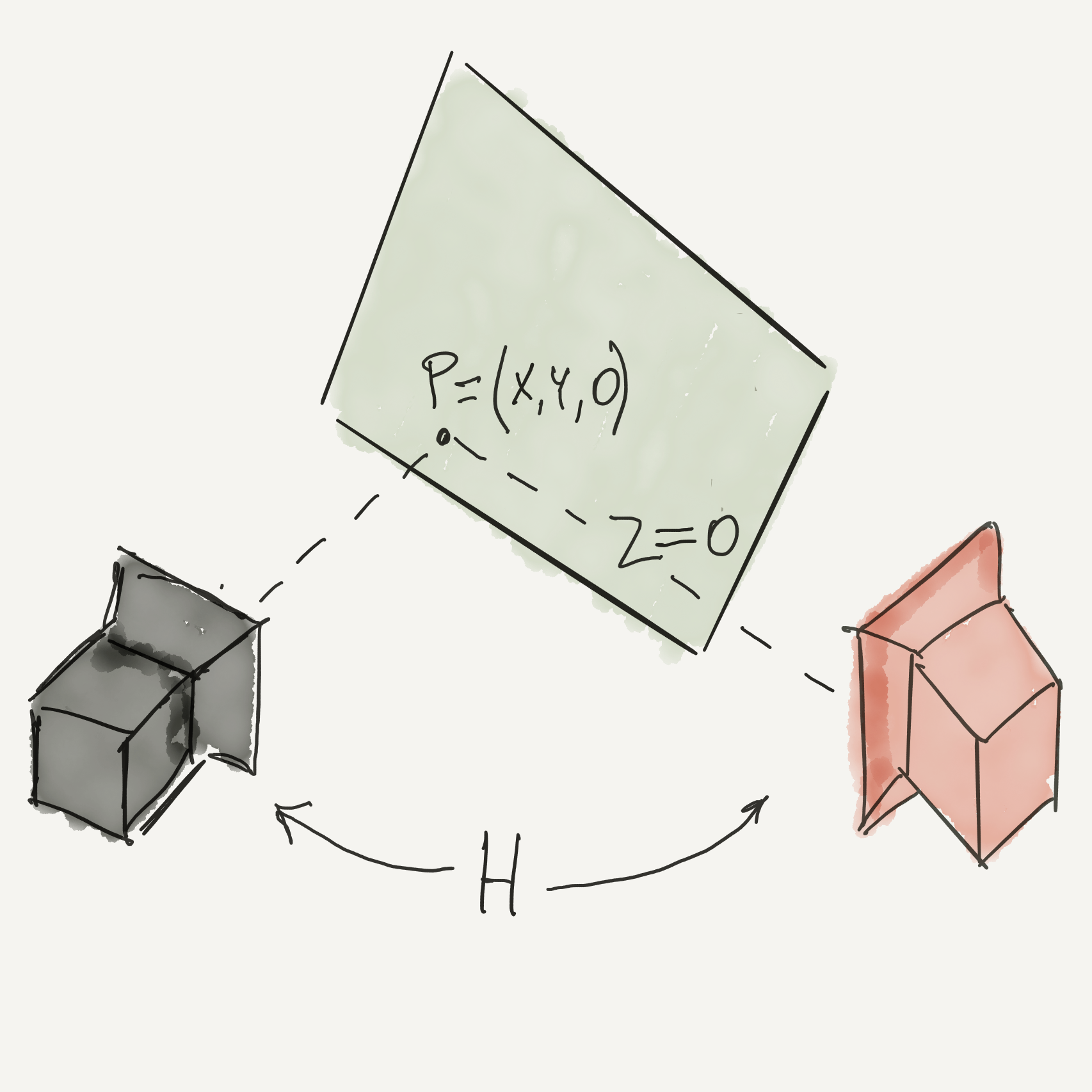
Now imagine a second camera, looking at the points on the same designated plane

We could do something like the following:from the first camera’s image plane, we could apply an inverse projection to get the points on the world plane, then project them on the second camera image plane by using its camera matrix. We could, in other words, combine the two transformations and obtain a single homography H, which will project co-planar points (in the world space) from one image to the other. Mind that this change of perspective will work only for points on that same plane, as the general case would need a 4x4 matrix M.

The mapping equation for the homography will be

Homography calculation

Even if H is the result of combining two camera matrices, you don’t need to know them to calculate H. There are 8 degrees of freedom, so you would need just 8 equations for the 8 unknowns. Those equations could be written by using 4 couples of corresponding points in the given images planes.

How do we obtain those equations? So, we have $\mathbb{x_1} \sim\ H\mathbb{x_2}$ for points on a plane in world space. Written explicitly:

Taking into account the fact that non-homogeneous coordinates are

then we can write

Rearranging the above, we get

And then

And then

Now, if we define the following three vectors

Then the above equations become simply

If we stack at least 8 equations, using 4 couples of corresponding points, then we can form the following linear system of equation

Well, we are basically done, as we can use tf.matrix_solve_ls to solve the linear system. Hereafter the code

def ax(p, q):   
    return [ p[0], p[1], -1, 0, 0, 0, -p[0] * q[0], -p[1] * q[0] ]
    
def ay(p, q):
    return [ 0, 0, 0, p[0], p[1], 1, -p[0] * q[1], -p[1] * q[1] ]

def homography(x1s, x2s):

    p = []
    
    # we build matrix A by using only 4 point correspondence. The linear
    # system is solved with the least square method, so here 
    # we could even pass more correspondence 
    p.append(ax(x1s[0], x2s[0]))
    p.append(ay(x1s[0], x2s[0]))

    p.append(ax(x1s[1], x2s[1]))
    p.append(ay(x1s[1], x2s[1]))   
    
    p.append(ax(x1s[2], x2s[2]))
    p.append(ay(x1s[2], x2s[2]))
   
    p.append(ax(x1s[3], x2s[3]))
    p.append(ay(x1s[3], x2s[3]))
    
    # A is 8x8
    A = tf.stack(p, axis=0)  
    
    m = [[x2s[0][0], x2s[0][1], x2s[1][0], x2s[1][1], x2s[2][0], x2s[2][1], x2s[3][0], x2s[3][1]]]

    # P is 8x1
    P = tf.transpose(tf.stack(m, axis=0))  
      
    # here we solve the linear system
    # we transpose the result for convenience
    return tf.transpose(tf.matrix_solve_ls(A, P, fast=True))

I also created a jupyter notebook on github as an example.

That’s all folks.